100 Ways to Kill Overfitting: Besides Data Augmentation, What Unconventional Solutions Can You Think Of?

In the brutal arena of deep learning, overfitting is not only the primary enemy of model training but also the watershed distinguishing junior parameter tuners from senior algorithm engineers. Although textbook "Dropout plus L2 regularization" theoretically establishes a basic defense, these traditional methods often fall short against over-parameterized modern models (such as Vision Transformer) and high-dimensional sparse data due to disrupting feature continuity or providing insufficient constraints. When validation Loss oscillates or severe distribution shifts occur between Public LB and Private LB, relying solely on Early Stopping is akin to self-deception and fails to reach the true ceiling of generalization. To reach the gold zone on Kaggle's fierce Leaderboard or break through in industrial small-sample SOTA rankings, we must introduce radical, mathematically intuitive "black magic." This involves manifold mixing strategies like Mixup and CutMix that break sample boundaries, Label Smoothing for decision boundaries, DropBlock for structural disruption of spatial correlations, and robustness gains from Adversarial Training. The core logic of modern SOTA solutions has shifted from explicit weight constraints to implicit regularization, using R-Drop's consistency constraints and Flooding's loss control to force models to learn robust global features rather than local noise. Mastering these niche yet efficient techniques demonstrates deep theoretical understanding in interviews and builds a defense mechanism beyond traditional paradigms, ensuring invincibility in the ultimate battle for generalization performance.

Why Standard "Dropout + L2" Is No Longer Enough?

If you are asked "how to prevent overfitting" in an interview, the standard textbook answer is usually: "Increase data size, use Dropout, add L2 regularization (weight decay), and Early Stopping." These methods indeed work well in classic machine learning tasks or simple fully connected networks, but when facing modern deep learning models (such as deep ResNet, Transformer) and highly competitive scenarios (such as Kaggle competitions or industrial small-sample SOTA sprints), this "old standard set" often appears inadequate.

Limitations of Traditional Methods

Standard regularization methods have obvious theoretical and practical shortcomings when facing over-parameterized modern models:

1. Ineffectiveness of Dropout: In Convolutional Neural Networks (CNNs), activation units in Feature Maps have extremely strong spatial correlation. Traditional Dropout randomly discards independent pixels or neurons; the network can still easily infer the missing information through adjacent activation units, leading to a significant discount in regularization effects. As pointed out in DropBlock research, only by discarding continuous "block" regions can the network be truly forced to learn more robust features rather than relying on local correlations.
2. The Ceiling of L2: L2 regularization essentially limits the norm of weights, assuming that "smaller weights mean a simpler model." However, the solution space of deep neural networks is extremely complex. Often, we need the model to maintain larger weights in certain dimensions to capture subtle features; pure weight compression might instead lead to underfitting or training difficulties.
3. Specifics of Kaggle Scenarios: In competitions or actual business, what we face is often not a simple "training set vs. test set" generalization problem, but the distribution shift between Public Leaderboard (LB) and Private LB. Relying solely on Early Stopping to monitor validation set Loss can easily lead to overfitting on the validation set or Public LB.

Explicit Regularization vs. Implicit Regularization

To understand why "niche" solutions are needed, we need to distinguish between two regularization logics:

• Explicit Regularization: Directly modifying the loss function or network structure, such as L2 (loss + lambda * w^2) or Dropout.
• Implicit Regularization: Achieving regularization effects by changing data distribution, the dynamic characteristics of optimization algorithms, or the training process. Examples include the noise introduced by SGD itself, the choice of Batch Size, and techniques like Mixup and Flooding that this article will focus on.

Modern SOTA solutions have shifted more towards operations at the data Manifold level and Loss Engineering, rather than simply putting locks on weights.

Core Defense System: From Beginner to "Black Tech"

To give you more ammunition when facing overfitting, we divide defense methods into "Basic" and "Advanced/Niche" categories. The following list aims to help you quickly build a knowledge index (Snippet-Ready):

• 🛡️ Basic Defense (Standard Methods)
• • Dropout: Randomly dropping neurons (limited effect on CNNs).
  • L1/L2 Regularization: Weight decay, parameter sparsification.
  • Early Stopping: Monitoring validation set metrics and stopping training at the right time.
  • Batch Normalization: Although mainly used to accelerate convergence, it also provides certain noise regularization effects.
  • Basic Data Augmentation: Rotation, cropping, flipping (preserving semantics only).
• 🚀 Advanced & Niche Solutions (Advanced & Niche Tricks)
• • Manifold Mixup Class (Manifold Mixup): Mixup, CutMix, breaking sample boundaries through linear interpolation.
  • Structural Dropout: DropBlock, regional dropping targeting CNN spatial correlation.
  • Loss Engineering: Label Smoothing, Flooding (preventing Training Loss from getting too low), Bi-Tempered Loss.
  • Adversarial Training: Adding tiny perturbations (FGSM/PGD) at the input layer to force model robustness against noise.
  • Self-Distillation & Consistency (Self-Distillation): R-Drop, forcing the outputs of two Dropout passes for the same sample to remain consistent.

In the following sections, we will skip those basic concepts you already know by heart and focus on breaking down those "niche" black technologies that can boost your score by 0.5% on the Leaderboard.

Data-Level "Black Tech": Beyond Simple Rotation and Flipping

In traditional deep learning engineering practice, data augmentation is often limited to geometric transformations (such as rotation, flipping, scaling) or photometric transformations (such as brightness adjustment). The core logic of these "classic" operations is Semantic Preserving: that is, the transformed images remain clearly recognizable as "cats" or "dogs" to the human eye, and the data points remain near the manifold of the original data distribution. However, when facing high-capacity models (such as EfficientNet, ViT) or extremely imbalanced datasets, relying solely on these mild perturbations is often insufficient to prevent the model from overfitting to specific textures or backgrounds.

Modern SOTA (State-of-the-Art) schemes and Kaggle champion solutions (such as those topping ImageNet or NLP leaderboards) have long introduced a class of more radical "black tech" augmentation strategies. Unlike traditional methods, these techniques—such as Mixing and Erasing strategies—intentionally destroy or blur the original semantics and physical structure of the samples.

According to the classification in arXiv:2212.10888, these methods construct training samples that are visually "unnatural" or even "unreadable" to humans by linearly interpolating pixels and labels, or by forcibly erasing key information regions. This seemingly counter-intuitive operation actually forces the model to abandon the rote memorization of local features, turning instead to learning more robust global features, and effectively smoothing the decision boundaries between classes. The following subsections will delve into these specific techniques that break sample boundaries and the mathematical intuition behind them.

Mixup and CutMix: Breaking the Boundaries Between Samples

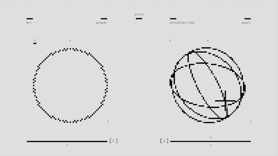
Traditional "Data Augmentation" methods such as rotation, cropping, or flipping essentially still perturb samples while maintaining a single primary semantic. Although this approach increases data diversity, the model often exhibits sharp transitions at the Decision Boundary between two classes—meaning the judgment from "cat" to "dog" might suddenly jump with minimal pixel changes, causing the model to appear vulnerable in the face of adversarial attacks or noise.

The emergence of Mixup and CutMix completely changed this logic: they no longer attempt to maintain a single semantic, but instead force the model to learn linear transition relationships on the empty manifold between samples by "forcibly fusing" two completely different samples.

Mixup: The Art of Linear Interpolation

Mixup's core intuition is very counter-intuitive: show the model a "ghost image" (e.g., a 70% transparent cat overlaid on a 30% transparent dog) and tell the model the label for this image is [0.7, 0.3].

From a mathematical perspective, Mixup performs simple linear interpolation between two random samples $(x_i, y_i)$ and $(x_j, y_j)$:

$$
\begin{aligned}
\tilde{x} &= \lambda xi + (1 - \lambda) xj \\
\tilde{y} &= \lambda yi + (1 - \lambda) yj
\end{aligned}
$$

Where $\lambda \in [0, 1]$ usually follows a Beta distribution $\text{Beta}(\alpha, \alpha)$.

Why is this "unnatural" data effective?
Mixup is actually executing a strategy called Vicinal Risk Minimization (VRM). It forces the model to establish a linear transition region between two classes, rather than a steep black-and-white boundary. This directly smooths the surface of the loss function, making gradient descent more stable, and significantly reduces the model's overconfidence in unknown data.

Here is a simple PyTorch implementation logic snippet:

# Mixup implementation snippet
alpha = 1.0
lam = np.random.beta(alpha, alpha)

# Mixed input
mixedx = lam  x + (1 - lam)  xshuffled
# Mixed labels (used when calculating Loss)
criterion = nn.CrossEntropyLoss()
loss = lam  criterion(pred, y) + (1 - lam)  criterion(pred, y_shuffled)

CutMix: Solving the Locality Problem of "Ghost Images"

Although Mixup is effective in image classification (ImageNet), it has a flaw: the generated images are visually unnatural blurry overlays, which may confuse the model regarding local features of the image (such as textures, edges).

CutMix proposes a mixing method that aligns better with human visual cognition: Cut and Paste.

CutMix does not change pixel values; instead, it "cuts" a random rectangular region from image B and pastes it onto the corresponding position of image A. The label mixing ratio $\lambda$ is no longer directly determined by a random distribution, but is strictly equal to the ratio of the cropped area to the total area.

The advantages of CutMix lie in:

1. Preserves local features: The patches in the image remain clear, natural object parts (e.g., a dog's head pasted on a cat's body), forcing the model to learn to recognize local features rather than relying on global statistical information.
2. Enhances localization capability: Since the model must predict probabilities based on the area of visible pixels, it is forced to focus on "where" the target is in the image, making CutMix perform better than Mixup in Object Detection and weakly supervised localization tasks.
3. Prevents information loss: Compared to Cutout, which directly removes a patch of pixels (resulting in complete information loss), CutMix fills the gap with information from another image, maintaining the strength of the training signal.

In Kaggle computer vision competitions (such as RSNA, Cassava Leaf Disease), CutMix and Mixup are almost standard features of Top solutions. They are not only regularization means to prevent overfitting but also "nuclear weapons" for improving model generalization capabilities. Especially in scenarios with limited data or Noisy Labels, models trained using Soft Labels are often more robust than those using Hard Labels.

Cutout, Random Erasing, and GridMask: Forcing the Model to "See the Whole Through a Tube"

If Mixup expands data boundaries by "mixing" information, then Cutout and its variants force model evolution by "subtraction." The underlying logic of these methods is very intuitive: If the model always fixates only on the dog's head to identify a dog, then we block the dog's head, forcing it to learn the dog's tail, fur color, or posture.

From "Simple and Crude" to "Sophisticated" Occlusion

In actual engineering, we usually go through the following evolutionary stages:

1. Cutout / Random Erasing:
   This is the most basic operation. A rectangular region is randomly selected in the image, and its pixel values are filled with 0 (black), 255 (white), or the dataset mean.

• • Intuition: Simulates object occlusion in real-world scenarios.
  • Effect: Significantly improves the model's Localization Ability. Because the model can no longer be lazy and look only at the most discriminative parts, it must pay attention to the overall context of the object.

1. GridMask:
   Cutout has a clear defect: for small objects or long-shot images, a random rectangular occlusion might completely cover the entire target. At this point, there is no "cat" in the picture, but the label remains "cat," which artificially creates noisy labels and misleads the model.

• • Improvement: GridMask no longer uses a single large color block but generates a grid-like mask (Grid Pattern).
  • Advantage: It preserves partial target information (through the gaps in the grid) while destroying feature continuity. This "severed but connected" approach avoids the risk of completely occluding the target while maintaining high-intensity regularization training for the model.

Pitfalls and Warnings in Engineering Practice

Although the code implementation of these methods is simple (usually just a few lines of Numpy or PyTorch Transform), they can easily fail in specific scenarios:

• Nightmare for Small Object Detection: On datasets like COCO that contain many tiny objects, be cautious when using large-area Random Erasing. If your target occupies only 1% of the screen, random erasing can easily cover it completely, leading to model training oscillation.
• Risk of Semantic Loss: Unlike Mixup, Cutout is destructive. When using it, it is recommended to use Bounding Box information for constraints—that is, restrict the occluded area from completely covering the Ground Truth Box, or adjust the proportion of the occluded area (e.g., limit it to within 10%-20% of the original image area).
• Training Duration: Since the difficulty of data recognition (Hard Examples) is artificially increased, the model often requires more Epochs to converge. If your computing budget is limited, you need to weigh this cost.

Summary: The core of these "viewing through a tube" methods lies in De-biasing. It forces the model to no longer rely on local textures but to learn more robust global shape features, making it a cost-effective means to improve model generalization ability.

Magic at the Label & Loss Function Level (Label & Loss Engineering)

After discussing "brute-force" data augmentations like Cutout and Mixup targeting the input end (Input Space), we need to turn our attention to the model's output end (Output Space). Often, overfitting does not stem from insufficient data volume, but rather from the overly absolute way we define the "correct answer" and the overly singular way we penalize errors.

In standard classification tasks, we are accustomed to using One-hot encoding as labels (e.g., [0, 1, 0]). This black-and-white labeling method implies a strong assumption: this image is "100%" a cat and "absolutely" not a dog. From a mathematical perspective, in order to bring the Cross-Entropy Loss down to an absolute 0, the Softmax function needs to output a probability of 1.0, which forces the model to push the Logits of the corresponding class towards positive infinity (Infinity).

This mechanism encourages the model to become "Overconfident." To achieve this extreme confidence, neural networks often overfit noise or non-robust features (such as background textures) in the training data, thereby sacrificing generalization ability. This chapter will explore how to implement regularization at the mathematical level by introducing "Soft Targets" or modifying the response mechanism of the loss function to "reduce confidence" in the model, thereby suppressing overfitting at the source.

Label Smoothing: Penalizing "Overconfidence"

In traditional classification tasks, we are accustomed to using One-Hot encoding (Hard Labels) as training targets: if an image is a "cat", due to the characteristics of Cross-Entropy Loss, the model will tend to make the Softmax output infinitely close to 1.0 in order to reduce the Loss to absolute 0. This forces the Logits (values before entering Softmax) to tend towards positive infinity.

This mechanism leads to the model becoming "overconfident": it not only memorizes the class but also attempts to fit every detail in the training data, including noise, by pushing up the weights.

The core idea of Label Smoothing is to dampen this confidence. It no longer demands the model to output perfect 1s and 0s, but instead "softens" the target distribution.

Mathematical Intuition and Implementation

We adjust the target probability from an absolute 1 to 1 - ε, and distribute the remaining ε probability evenly among all classes (including the correct class itself, or only among the incorrect classes, depending on the specific implementation).

The formula is usually as follows:

For example, in a three-class classification task, the standard Hard Label is [0, 1, 0]. After smoothing with $\epsilon=0.1$, the target becomes [0.033, 0.933, 0.033].
This is actually telling the model: "Although this image is highly likely to be Class B, don't be too absolute; leave some room for other possibilities."

Why Does It Prevent Overfitting?

1. Limiting Weight Explosion: Since the target probability is no longer 1, the model does not need to push Logits to infinity to reach the optimal solution. Mathematically, this limits the norm of the weights, acting similarly to L2 regularization.
2. Tolerance to Noise: As pointed out in Label Smoothing Explained, this method keeps the model "humble". When there are incorrect labels (Noisy Labels) in the training data, Hard Labels force the model to fit the wrong Ground Truth, while Soft Labels reduce the compulsiveness of this erroneous signal.
3. Better Calibration: Studies show that models trained with label smoothing produce predicted probabilities that better reflect true accuracy (lower Expected Calibration Error).

Applicable Scenarios and Engineering Suggestions

• Default Choice for Transformers: In the training scripts of BERT, Transformer, and many SOTA image classification models (such as EfficientNet), Label Smoothing has become almost a standard configuration.
• When Data Noise is High: If you suspect that the annotation quality of the dataset is not high (e.g., data obtained via web crawling), Label Smoothing is a more direct defense mechanism than Dropout.
• Comparison with Hard Labels:
• • Hard Labels: Suitable for simple tasks where boundaries between classes are extremely distinct and annotations are absolutely accurate.
  • Soft Labels: Suitable for scenarios with many classes, high feature overlap, or where better model generalization is desired.

Note: Label Smoothing also has side effects. It forcibly suppresses the probability of the correct class, which may lead to insufficient intra-class distance in certain retrieval tasks requiring extremely high confidence thresholds. However, in pure classification tasks, it is usually a safe bet.

Bi-Tempered Loss and Focal Loss: Focusing on Hard Examples

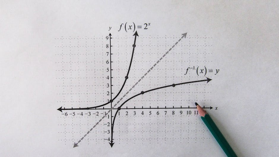
When dealing with overfitting problems, we are usually accustomed to imposing constraints "externally" (such as Dropout or L2 regularization), but often overlook the role of the Loss Function itself in shaping model training dynamics. Standard Cross Entropy (CE) Loss, when faced with a large number of simple samples, often sees its accumulated gradients dominate the optimization direction, causing the model to overfit in the "comfort zone" while ignoring the Hard Examples that truly determine generalization ability. Meanwhile, CE is overly sensitive to Outliers, easily forcibly fitting noisy labels.

By replacing the loss function, we can achieve "implicit regularization," reshaping the model's learning preferences at the Optimization Landscape level.

Focal Loss: Not Just for Object Detection

Although Focal Loss was originally proposed to solve the extreme positive-negative sample imbalance problem in One-Stage Object Detection, it is also an excellent regularization method in classification tasks.

Focal Loss introduces a modulating factor $(1 - p_t)^\gamma$ on top of standard CE. Its core mechanism lies in dynamically adjusting sample weights:

• Reduce weight of simple samples: When the model is very confident about a sample ($p_t \rightarrow 1$), this modulating factor approaches 0. This means the gradient contribution generated by simple samples that have already been "learned" by the model will be significantly weakened.
• Mine hard samples: The model is forced to focus its attention on those "hard" samples with lower predicted probabilities.

From the perspective of overfitting, Focal Loss prevents the model from becoming Overconfident in the later stages of training in order to further reduce the Loss of simple samples; this overconfidence is often a precursor to overfitting. It acts as a kind of "soft" Hard Negative Mining, forcing the model to learn the boundaries of the data distribution rather than rote memorizing easily identifiable features.

Bi-Tempered Logistic Loss: Handling Noise and Outliers

If Focal Loss solves the problem of "learning too easily," the Bi-Tempered Logistic Loss proposed by Google solves the problem of "learning too indiscriminately." In many real-world scenarios or Kaggle competitions, datasets often contain Noisy Labels or outliers. Standard CE Loss is unbounded; to fit an erroneous outlier, the model may generate huge gradients, leading to severe distortion of the decision boundary, thereby triggering serious overfitting.

Bi-Tempered Loss introduces two "temperature" parameters ($t_1$ and $t_2$) to bidirectionally constrain the Loss:

1. Temperature $t_1$ (Tail Heavy-Tailing): By adjusting the logarithmic function, it provides Boundedness when dealing with outliers. This means that even when facing extremely absurd samples, the Loss will not increase infinitely, thereby limiting the destructive power of a single noise sample on the gradients.
2. Temperature $t_2$ (Softmax Smoothing): By adjusting the exponential function, it gives the probability distribution heavy-tailed characteristics, retaining more inter-class uncertainty, playing a role similar to Label Smoothing.

Engineering Practice Suggestions:
When your overfitting is caused by the dataset containing 10%~20% noisy labels (such as crawled data), directly using Bi-Tempered Loss is often more effective than simply increasing Dropout or data augmentation. It is essentially a noise-robust loss function that allows the model to "safely ignore" those data points that cannot be explained by normal logic during the training process, thereby maintaining the smoothness of the decision boundary.

"Disruption" of Network Structure and Training Dynamics (Structural & Adversarial)

If L2 regularization and Early Stopping are considered "gentle persuasion" for the model, then the techniques covered in this chapter are more like "brute-force special training." In the engineering practice of top-ranking Kaggle solutions and SOTA papers, relying solely on data augmentation often hits a ceiling. Consequently, experienced algorithm engineers have begun to introduce more destructive mechanisms at the levels of network structure and training dynamics.

The core logic of such methods is not merely to increase randomness, but to artificially create "worst-case scenarios" or "structural absences" during the training process. This is achieved through dynamic reconfiguration of the network topology (such as spatial masking targeting convolutional features) or deep intervention in the training loop (such as gradient-based adversarial attacks). This strategy of "seeking survival through destruction" forces the model to abandon reliance on local noise and shortcut features (Shortcut Learning), turning instead to capture more robust global features. The following content will explore how to introduce strong regularization effects brought about by "destruction" within the architecture and training flow.

对抗训练 (Adversarial Training / FGM / PGD)：Fighting Poison with Poison

In the perception of most engineers, Adversarial Examples usually belong to the category of security defense, used to prevent models from malicious attacks. However, in top-tier Kaggle solutions (especially NLP tasks) and SOTA papers, adversarial training has long since transformed into an ultimate regularization method.

If data augmentation is randomly "expanding" samples, then adversarial training is directionally "manufacturing" the hardest samples. Its core logic lies in the Min-Max Game: during the training process, first find the perturbation (Attack) that maximizes the current Loss via gradient ascent, then let the model minimize the Loss under this "worst-case scenario" (Defense). Through this method of "fighting poison with poison," it forces the model to smooth decision boundaries, thereby significantly improving generalization capabilities.

Core Algorithms: From FGM to PGD

In engineering implementation, adversarial training is mainly divided into two steps: generating perturbations and updating parameters. Depending on the strategy for generating perturbations, there are two main streams:

1. FGM (Fast Gradient Method)
   Based on the improvement of FGSM proposed by Ian Goodfellow in 2014. It assumes the loss function is linear and obtains adversarial perturbations through a single gradient calculation.

• • Features: Fast calculation speed, requires only one backpropagation to generate perturbations.
  • Application: In NLP tasks, perturbations are usually applied to the Embedding layer (rather than directly modifying pixels like in CV). FGM is often used as the preferred Baseline method due to its efficiency.

1. PGD (Projected Gradient Descent)
   Proposed by Madry et al. in 2017, considered the "strongest first-order attack method." Essentially an iterative version of FGM: it performs multi-step small-step gradient ascent, projecting the perturbation back into the allowable perturbation range (e.g., $\epsilon$-ball) at every step.

• • Features: Generates higher quality adversarial samples with stronger aggressiveness, forcing the model to learn more robust features.
  • Application: In scenarios requiring extremely high precision, PGD can often squeeze out more score than FGM, but at the cost of multiplied computational volume.

Engineering Implementation Differences: In the CV field, perturbations are added to input pixels; whereas in NLP, since discrete Tokens cannot be differentiated, perturbations are usually added to the continuous vectors in the Word Embedding layer.

Costs and Trade-offs

Although adversarial training is called a "Killer Trick," it is not a free lunch. Introducing adversarial training will significantly alter the dynamics of the training loop:

• Explosion in training time: This is the most direct pain point. Using FGM requires one extra backpropagation to calculate perturbations, usually increasing training time by 2x; while using K-step iterative PGD, training time may increase by (K+1)x or even more.
• Difficult to converge: Since the model is constantly training on "worst-case samples," the Loss curve may exhibit violent oscillations.
• Capacity threshold: Adversarial training forces the model to learn more complex boundaries, which usually requires the model to have larger capacity. Forcing the use of PGD on small models may even lead to underfitting.

Nevertheless, in scenarios with limited data volume or where the model is extremely prone to overfitting, the regularization effect provided by adversarial training is often superior to Dropout and L2 weight decay. For developers wishing to quickly verify or integrate this technology, one can directly refer to mature implementation libraries, such as TorchAttacks, which encapsulates multiple attack strategies including PGD and FGM, and can be embedded into PyTorch training loops with standardized interfaces.

DropBlock and Stochastic Depth: Evolved Versions of Dropout

When dealing with Convolutional Neural Networks (CNNs), many engineers encounter a counter-intuitive phenomenon: classic Dropout often yields unsatisfactory results, or even fails to work at all. This is not a mystery, but rather because convolutional features possess high Spatial Correlation.

In fully connected layers, neurons are relatively independent, and randomly dropping certain nodes can effectively break Co-adaptation. However, on the Feature Maps of convolutional layers, adjacent activation units usually share extremely similar semantic information. If you simply randomly "turn off" a few pixels, the network can easily "infer" the missing information from the immediately surrounding pixels, causing the regularization effect to be greatly compromised.

To solve this problem, we need a more aggressive "evolved version" of Dropout.

1. DropBlock: From "Dead Pixels" to "Occlusion"

The core idea of DropBlock is very intuitive: since the loss of single pixels cannot stump the network, then directly drop a whole continuous region.

We can use a simple metaphor to understand the difference between the two:

• Standard Dropout is like a few random Dead Pixels on an image sensor. The network takes a look at the surrounding pixels and can easily mentally fill in the content of the dead pixels, requiring almost no change in its learning strategy.
• DropBlock is like someone casually stuck a Post-it Note on the image. This Post-it note might directly cover the "dog head," forcing the network to learn to recognize the "dog tail," "fur texture," or "leg shape" and other features to complete the classification.

This method forces the network to no longer rely on a single Discriminative Feature, but to search for more diverse evidence, thereby significantly improving the model's generalization ability. Relevant technical discussions also point out that DropBlock's regularization effect on spatial data is far stronger than random Dropout, because it truly introduces the challenge of information loss.

2. Stochastic Depth: Subtraction in the Depth Dimension

If DropBlock operates on "width" and "space," then Stochastic Depth performs subtraction on "depth," specifically targeting deep residual networks like ResNet.

When training extremely deep networks (such as ResNet-101 or ResNet-152), Stochastic Depth will randomly Bypass entire Residual Blocks with a certain probability. This means:

1. During Training: In every iteration, the network is actually training a random "shallow sub-network." Since the path is shorter, the gradient vanishing problem is alleviated, and training speed also increases.
2. During Testing: The complete deep network is used. This is equivalent to performing an Implicit Ensemble of countless shallow networks of different depths.

Engineering Advice:
In modern vision tasks (especially Kaggle competitions or high-precision industrial scenarios), if you are using ResNet, ResNeXt, or EfficientNet variants, it is recommended to prioritize DropBlock or Stochastic Depth rather than forcibly inserting traditional Dropout layers after convolutional layers. The former preserves the essence of Dropout's "model ensemble" while avoiding the failure issues caused by the redundancy of convolutional features.

Interviewer's Perspective: How to Answer "Preventing Overfitting" for a High Score?

When an interviewer throws out the classic question "how to prevent overfitting," they usually do not expect a textbook-style list of nouns (such as "Dropout, L2 regularization, Data Augmentation"), but rather whether you can demonstrate systematic engineering thinking and the ability to make trade-offs for specific scenarios.

Merely reciting standard rote answers will only get you a passing grade; to get a high score, you need to structure your answer and actively point out "the limitations of traditional methods in modern deep learning." Here is a suggested answer framework and strategy.

1. Reject "Rote Listing," Build a Layered Defense System

A high-scoring answer should be like building a fortification, elaborated in layers from the data source to the model output. It is recommended to organize your language using the following logic:

• Data Level (Root Cause Governance): Emphasize that data is the fundamental solution to overfitting. Beyond conventional rotation and cropping, focus on mentioning modern augmentation methods like Mixup or CutMix. Research shows that Mix-based data augmentation methods often improve model generalization boundaries more than traditional augmentation, especially in physiological time series or image classification tasks.
• Model Level (Structural Constraints): Mention the control of model Capacity. Here you can naturally introduce DropBlock or Stochastic Depth, explaining why they are more effective than standard Dropout in ResNet or Transformer architectures.
• Training Level (Process Intervention): Mention Early Stopping and Adversarial Training.
• Label Level (Target Smoothing): Mention Label Smoothing to prevent the model from being overconfident about incorrect labels.

2. Demonstrate "Senior" Perspective Trade-offs (It Depends)

The difference between a senior engineer and a beginner lies in their sensitivity to context. After listing methods, you must add a discussion on "specific usage depends on the scenario":

• Conflict between Batch Norm and Dropout: Don't just mention L2 regularization. Point out that in modern networks using Batch Normalization (BN), traditional Dropout may lead to variance shifts, often resulting in suboptimal performance. In this case, priority should be given to Weight Decay or regularization methods specifically for convolutional layers.
• Pitfalls of Validation Strategies: Preventing overfitting is not just about "what was done during training," but also "how to evaluate." Citing experience from Kaggle competitions, always trusting your Cross-Validation (CV) score is often more important than staring at the public Leaderboard. Many beginners over-optimize the LB score and eventually crash on the private set, which itself is a typical case of "overfitting to the test set."

3. Pitfall Avoidance Guide: Don't Theorize for the Sake of Theory

A common point deduction in interviews is applying mathematical explanations mechanically while ignoring engineering reality. For example:

• Be cautious when talking about L1 Regularization Sparsity: Although theoretically L1 can produce sparse weights, in the SGD optimization of modern deep learning frameworks (like PyTorch/TensorFlow), true sparsification is hard to achieve through simple L1 unless combined with specialized Pruning algorithms.
• Dialectics of Data Volume and Noise: If the data volume is extremely small and noise is high, simple Oversampling might exacerbate overfitting; mentioning Transfer Learning or Freezing Layers is a more relevant solution in this context.

Example Summary Script:

"There is no silver bullet for preventing overfitting. If it is a small-sample image task, I would prioritize Transfer Learning and CutMix; if it is structured data, I would focus more on feature selection and the consistency of the CV strategy. The core principle is: find the optimal balance point between Bias and Variance under the current data scale."